%pylab inline
import numpy as np
import scipy.signal as dsp
from palettable.colorbrewer.qualitative import Dark2_8

colors = Dark2_8.mpl_colors
rst = np.random.RandomState(1)
Populating the interactive namespace from numpy and matplotlib
Design of a digital deconvolution filter (FIR type)
from PyDynamic.deconvolution.fit_filter import LSFIR_unc
from PyDynamic.misc.SecondOrderSystem import *
from PyDynamic.misc.testsignals import shocklikeGaussian
from PyDynamic.misc.filterstuff import kaiser_lowpass, db
from PyDynamic.uncertainty.propagate_filter import FIRuncFilter
from PyDynamic.misc.tools import make_semiposdef
# parameters of simulated measurement
Fs = 500e3
Ts = 1 / Fs

# sensor/measurement system
f0 = 36e3; uf0 = 0.01*f0
S0 = 0.4; uS0= 0.001*S0
delta = 0.01; udelta = 0.1*delta

# transform continuous system to digital filter
bc, ac = sos_phys2filter(S0,delta,f0)
b, a = dsp.bilinear(bc, ac, Fs)

# Monte Carlo for calculation of unc. assoc. with [real(H),imag(H)]
f = np.linspace(0, 120e3, 200)
Hfc = sos_FreqResp(S0, delta, f0, f)
Hf = dsp.freqz(b,a,2*np.pi*f/Fs)[1]

runs = 10000
MCS0 = S0 + rst.randn(runs)*uS0
MCd  = delta+ rst.randn(runs)*udelta
MCf0 = f0 + rst.randn(runs)*uf0
HMC = np.zeros((runs, len(f)),dtype=complex)
for k in range(runs):
    bc_,ac_ = sos_phys2filter(MCS0[k], MCd[k], MCf0[k])
    b_,a_ = dsp.bilinear(bc_,ac_,Fs)
    HMC[k,:] = dsp.freqz(b_,a_,2*np.pi*f/Fs)[1]

H = np.r_[np.real(Hf), np.imag(Hf)]
uAbs = np.std(np.abs(HMC),axis=0)
uPhas= np.std(np.angle(HMC),axis=0)
UH= np.cov(np.hstack((np.real(HMC),np.imag(HMC))),rowvar=0)
UH= make_semiposdef(UH)
Problem description
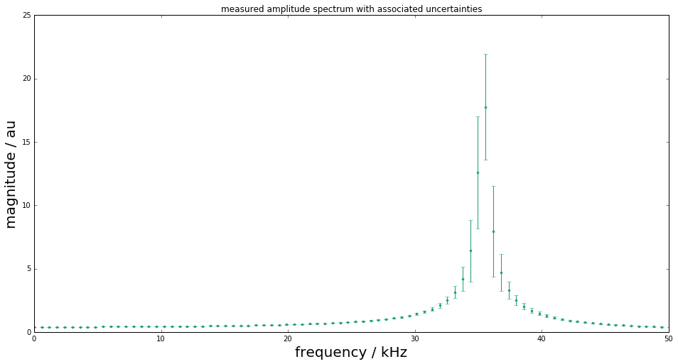
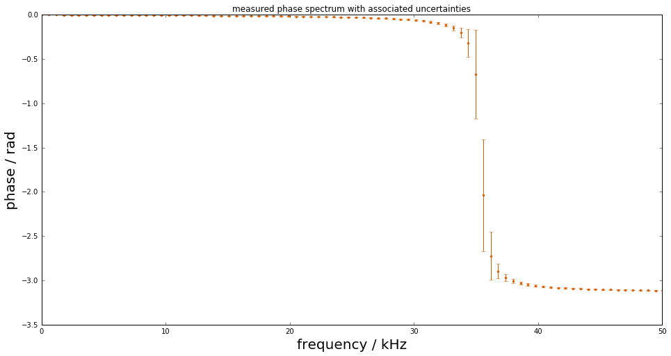
Assume information about a linear time-invariant (LTI) measurement system to be available in terms of its frequency response values \(H(j\omega)\) at a set of frequencies together with associated uncertainties:
figure(figsize=(16,8))
errorbar(f*1e-3, np.abs(Hf), uAbs, fmt=".", color=colors[0])
title("measured amplitude spectrum with associated uncertainties")
xlim(0,50)
xlabel("frequency / kHz",fontsize=20)
ylabel("magnitude / au",fontsize=20);
figure(figsize=(16,8))
errorbar(f*1e-3, np.angle(Hf), uPhas, fmt=".", color=colors[1])
title("measured phase spectrum with associated uncertainties")
xlim(0,50)
xlabel("frequency / kHz",fontsize=20)
ylabel("phase / rad",fontsize=20);
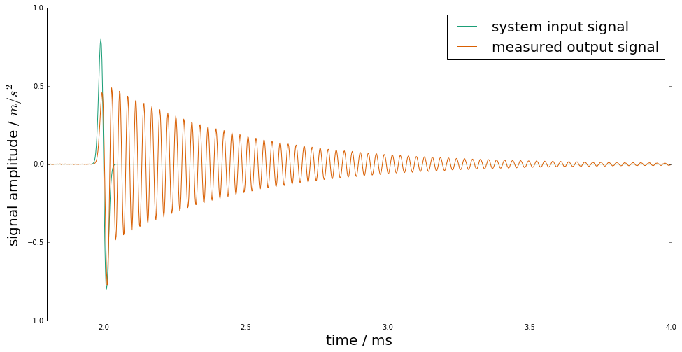
Simulated measurement
Measurements with this system are then modeled as a convolution of the system’s impulse response
with the input signal \(x(t)\), after an analogue-to-digital conversion producing the measured signal
# simulate input and output signals
time = np.arange(0, 4e-3 - Ts, Ts)
#x = shocklikeGaussian(time, t0 = 2e-3, sigma = 1e-5, m0=0.8)
m0 = 0.8; sigma = 1e-5; t0 = 2e-3
x = -m0*(time-t0)/sigma * np.exp(0.5)*np.exp(-(time-t0) ** 2 / (2 * sigma ** 2))
y = dsp.lfilter(b, a, x)
noise = 1e-3
yn = y + rst.randn(np.size(y)) * noise
figure(figsize=(16,8))
plot(time*1e3, x, label="system input signal", color=colors[0])
plot(time*1e3, yn,label="measured output signal", color=colors[1])
legend(fontsize=20)
xlim(1.8,4); ylim(-1,1)
xlabel("time / ms",fontsize=20)
ylabel(r"signal amplitude / $m/s^2$",fontsize=20);
Design of the deconvolution filter
The aim is to derive a digital filter with finite impulse response (FIR)
such that the filtered signal
<<<<<<< HEAD is an estimate of the system’s input signal at the discrete time points ======= is an estimate of the system’s input signal at the discrete time points. >>>>>>> devel1
Publication
- Elster and Link “Uncertainty evaluation for dynamic measurements modelled by a linear time-invariant system” Metrologia, 2008
- Vuerinckx R, Rolain Y, Schoukens J and Pintelon R “Design of stable IIR filters in the complex domain by automatic delay selection” IEEE Trans. Signal Process. 44 2339–44, 1996
Determine FIR filter coefficients such that
with a pre-defined time delay \(n_0\) to improve the fit quality (typically half the filter order).
Consider as least-squares problem
with - \(y\) real and imaginary parts of the reciprocal and phase shifted measured frequency response values - \(X\) the model matrix with entries \(e^{-j k \omega/Fs}\) - \(b\) the sought FIR filter coefficients - \(W\) a weighting matrix (usually derived from the uncertainties associated with the frequency response measurements
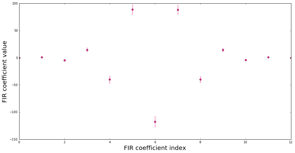
Filter coefficients and associated uncertainties are thus obtained as
# Calculation of FIR deconvolution filter and its assoc. unc.
N = 12; tau = N//2
bF, UbF = deconv.LSFIR_unc(H,UH,N,tau,f,Fs)
Least-squares fit of an order 12 digital FIR filter to the
reciprocal of a frequency response given by 400 values
and propagation of associated uncertainties.
Final rms error = 1.545423e+01
figure(figsize=(16,8))
errorbar(range(N+1), bF, np.sqrt(np.diag(UbF)), fmt="o", color=colors[3])
xlabel("FIR coefficient index", fontsize=20)
ylabel("FIR coefficient value", fontsize=20);
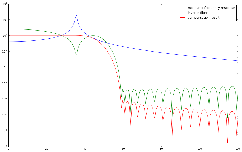
In order to render the ill-posed estimation problem stable, the FIR inverse filter is accompanied with an FIR low-pass filter.
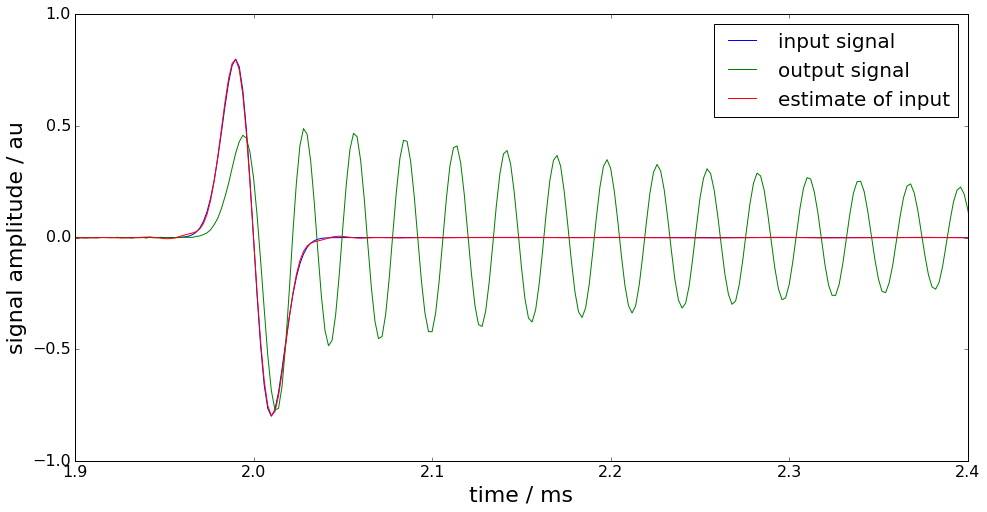
Application of the deconvolution filter for input estimation is then carried out as
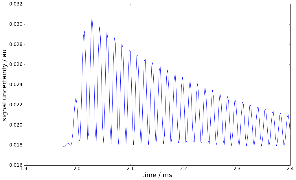
with point-wise associated uncertainties calculated as
fcut = f0+10e3; low_order = 100
blow, lshift = kaiser_lowpass(low_order, fcut, Fs)
shift = -tau - lshift
figure(figsize=(16,10))
HbF = dsp.freqz(bF,1,2*np.pi*f/Fs)[1]*dsp.freqz(blow,1,2*np.pi*f/Fs)[1]
semilogy(f*1e-3, np.abs(Hf), label="measured frequency response")
semilogy(f*1e-3, np.abs(HbF),label="inverse filter")
semilogy(f*1e-3, np.abs(Hf*HbF), label="compensation result")
legend();
xhat,Uxhat = FIRuncFilter(yn,noise,bF,UbF,shift,blow)
figure(figsize=(16,8))
plot(time*1e3,x, label='input signal')
plot(time*1e3,yn,label='output signal')
plot(time*1e3,xhat,label='estimate of input')
legend(fontsize=20)
xlabel('time / ms',fontsize=22)
ylabel('signal amplitude / au',fontsize=22)
tick_params(which="both",labelsize=16)
xlim(1.9,2.4); ylim(-1,1);
figure(figsize=(16,10))
plot(time*1e3,Uxhat)
xlabel('time / ms',fontsize=22)
ylabel('signal uncertainty / au',fontsize=22)
subplots_adjust(left=0.15,right=0.95)
tick_params(which='both', labelsize=16)
xlim(1.9,2.4);
Basic workflow in PyDynamic
Fit an FIR filter to the reciprocal of the measured frequency response
from PyDynamic.deconvolution.fit_filter import LSFIR_unc
bF, UbF = LSFIR_unc(H,UH,N,tau,f,Fs, verbose=False)
with - H the measured frequency response values - UH the
covariance (i.e. uncertainty) associated with real and imaginary parts
of H - N the filter order - tau the filter delay in samples -
f the vector of frequencies at which H is given - Fs the
sampling frequency for the digital FIR filter
Propagate the uncertainty associated with the measurement noise and the FIR filter through the deconvolution process
xhat,Uxhat = FIRuncFilter(yn,noise,bF,UbF,shift,blow)
with - yn the noisy measurement - noise the std of the noise -
shift the total delay of the FIR filter and the low-pass filter -
blow the coefficients of the FIR low-pass filter